Machine learning (sometimes abbreviated to ML) is a class of statistical tools that help analysts find patterns in data. Basically, ML helps with prediction problems. Many core methods in ML are modern, with new developments everyday, but there are also fundamental components that have been around for a long time and now can be applied thanks to the larger availability of large datasets and computing power. Academic researchers use ML but it is also commonly used in the public and private sectors, and is a core part of recent advances in AI tools. We will go through some ML basics and see how to implement them in R. You will have practice doing so with an activity.
There are two broad categories of ML.
Supervised learning. Here there is an explicit outcome the analyst uses for prediction. For example, if the analyst observes historic house prices and housing characteristics and they want to predict future house prices. The outcome “house prices” is observed in some of the data and used in estimation.
Unsupervised learning. In this case, the outcome is not used for estimation. For example, the analyst may want to group the houses in the data into clusters of similar houses. They do not have any idea of what these clusters are and there is no indication of them in the data. ML tools can still provide a way to do this!
21.1 Supervised Learning
21.1.1 Linear Regression
You already are familiar with a method that can be used for prediction. Before, we were using linear regression to understand the relationship between the outcome variable (\(Y\)) and covariates (\(X_1, X_2, \ldots\)). Now, instead of focusing on interpreting the coefficients, we focus on minimizing prediction error. Specifically, linear regression minimizes the mean squared error (MSE) between the predicted and observed outcomes. If the fitted value is \(\hat{Y}_i\), the MSE is
Consider two datasets. One is the training dataset. We use this dataset to estimate the linear regression. From this dataset, we get the estimated coefficients. In the testing dataset we predict the outcome but using the estimated coefficients from the training dataset. Because we actually observe the outcome in tthe testing dataset as well, we can compute the squared prediction error. Suppose we have one dataset that we partition into training \((i = 1, 2, \ldots, N)\) and testing \((i = N+1, N+2, \ldots, M)\) datasets.
Let us see how we implement this in R. We will use a dataset from the ggplot2 package called diamonds. This is a very clean dataset with the price and attribute of diamonds. We will try to predict the price of diamonds based on their attributes. You can think of this exercise extending to any situation where you want to predict prices.
library(ggplot2)library(dplyr)
Attaching package: 'dplyr'
The following objects are masked from 'package:stats':

    filter, lag
The following objects are masked from 'package:base':

    intersect, setdiff, setequal, union
library(magrittr)data(diamonds)summary(diamonds)
     carat               cut        color        clarity          depth
 Min.   :0.2000   Fair     : 1610   D: 6775   SI1    :13065   Min.   :43.00
 1st Qu.:0.4000   Good     : 4906   E: 9797   VS2    :12258   1st Qu.:61.00
 Median :0.7000   Very Good:12082   F: 9542   SI2    : 9194   Median :61.80
 Mean   :0.7979   Premium  :13791   G:11292   VS1    : 8171   Mean   :61.75
 3rd Qu.:1.0400   Ideal    :21551   H: 8304   VVS2   : 5066   3rd Qu.:62.50
 Max.   :5.0100                     I: 5422   VVS1   : 3655   Max.   :79.00
                                    J: 2808   (Other): 2531
     table           price             x                y
 Min.   :43.00   Min.   :  326   Min.   : 0.000   Min.   : 0.000
 1st Qu.:56.00   1st Qu.:  950   1st Qu.: 4.710   1st Qu.: 4.720
 Median :57.00   Median : 2401   Median : 5.700   Median : 5.710
 Mean   :57.46   Mean   : 3933   Mean   : 5.731   Mean   : 5.735
 3rd Qu.:59.00   3rd Qu.: 5324   3rd Qu.: 6.540   3rd Qu.: 6.540
 Max.   :95.00   Max.   :18823   Max.   :10.740   Max.   :58.900

       z
 Min.   : 0.000
 1st Qu.: 2.910
 Median : 3.530
 Mean   : 3.539
 3rd Qu.: 4.040
 Max.   :31.800
# Make the factors unordered (makes the regression easier)diamonds <- diamonds %>%mutate(across(c(cut, color, clarity), ~factor(.x, ordered =FALSE)))
Let us first define the training and testing datasets. We can randomly divide the data into the two datasets. We use 70% for the training dataset because we have a really big sample here.
set.seed(470500)# Create an ID variablediamonds <- diamonds %>%mutate(id =1:nrow(diamonds))# Randomly select 70% to the training datasettrain_ids <-sample(diamonds$id, size =0.7*nrow(diamonds))train <- diamonds[(diamonds$id %in% train_ids), ]test <- diamonds[!(diamonds$id %in% train_ids), ]
Now, we can use the training dataset to estimate the regression of price on characteristics.
train_lm <-lm(price ~ carat + cut + color + clarity + depth + table + x + y + z,data = diamonds)summary(train_lm)
Comparing the MSE between these two models, the first model has better predictive power. But what about other models? What about all the possible combinations of covariates? What about adding polynomials of those covariates? ML methods can help with that too (below).
21.1.2 Logistic Regression
We can apply the same logic when the outcome is binary, but we use logistic regression. The model predicts the probability of success, when the outcome is one. Suppose we want to predict if a diamond has a price below someone’s budget of $1,000.
train <- train %>%mutate(inbudget = (price <=1000))test <- test %>%mutate(inbudget = (price <=1000))# Trainib_train_lm <-glm(inbudget ~ carat + cut + color + clarity + depth + table + price + x + y + z,data = train,family ="binomial")
Warning: glm.fit: algorithm did not converge
Warning: glm.fit: fitted probabilities numerically 0 or 1 occurred
Under that intuition, ML methods can help us find a model (what to put on the right-hand side) for the best prediction (what is on the left-hand side). We will go through the workflow of LASSO, which is one method you can use.
Split the cleaned data into training and testing. We can use the tidymodels library to split the data into training and testing datsaets.
d_split <-initial_split(diamonds) # Creates the split (default is 75/25)d_train <-training(d_split) # Define training data based on splitd_test <-testing(d_split) # Definet testing data based on split
Build a “recipe.” This tells R what is the outcome variable and helps format the possible predictors.
recipe(price ~ ., data = d_train) %>%summary()
# A tibble: 11 × 4
   variable type      role      source
   <chr>    <list>    <chr>     <chr>
 1 carat    <chr [2]> predictor original
 2 cut      <chr [3]> predictor original
 3 color    <chr [3]> predictor original
 4 clarity  <chr [3]> predictor original
 5 depth    <chr [2]> predictor original
 6 table    <chr [2]> predictor original
 7 x        <chr [2]> predictor original
 8 y        <chr [2]> predictor original
 9 z        <chr [2]> predictor original
10 id       <chr [2]> predictor original
11 price    <chr [2]> outcome   original
# Account for ID variable and factor variablesd_rec <-recipe(price ~ ., data = d_train) %>%step_dummy(all_nominal_predictors()) %>%update_role(id, new_role ="ID") summary(d_rec)
# A tibble: 11 × 4
   variable type      role      source
   <chr>    <list>    <chr>     <chr>
 1 carat    <chr [2]> predictor original
 2 cut      <chr [3]> predictor original
 3 color    <chr [3]> predictor original
 4 clarity  <chr [3]> predictor original
 5 depth    <chr [2]> predictor original
 6 table    <chr [2]> predictor original
 7 x        <chr [2]> predictor original
 8 y        <chr [2]> predictor original
 9 z        <chr [2]> predictor original
10 id       <chr [2]> ID        original
11 price    <chr [2]> outcome   original
“Prep” the recipe. Given the recipe, R then puts together the data inputs. You can explore the outputs of recipe and prep to better understand these steps.
d_prep <- d_rec %>%prep()summary(d_rec)
# A tibble: 11 × 4
   variable type      role      source
   <chr>    <list>    <chr>     <chr>
 1 carat    <chr [2]> predictor original
 2 cut      <chr [3]> predictor original
 3 color    <chr [3]> predictor original
 4 clarity  <chr [3]> predictor original
 5 depth    <chr [2]> predictor original
 6 table    <chr [2]> predictor original
 7 x        <chr [2]> predictor original
 8 y        <chr [2]> predictor original
 9 z        <chr [2]> predictor original
10 id       <chr [2]> ID        original
11 price    <chr [2]> outcome   original
Specify parameters of the model. The basic idea of model selection is that we have an objective function with a penalty term. This penalty term depends on the number of predictors. If we include more predictors, the penalty increases. This prevents us just using every predictor available. Then the question is what parameters do we choose for our objective function? Here is the general format for LASSO:
We can dissect this term by term. The first term in Equation (1) is the usual OLS estimator. The second term is the penalty. The parameter \(\lambda\) is the first parameter we need to set. This itself is called the penalty term. Large values of \(\lambda\) results in a more parsimonious model (fewer predictors) because the penalty is large. If \(\lambda\) is zero, then the model is the same as OLS. In practice, they can cover a large range. See methods in cross-validation to select \(\lambda\) in a more principled way than just setting it. Then, there is the function on the parameters \(\beta\). Suppose there are \(K\) possible predictors. LASSO involves taking the absolute value of the parameters. Other methods, like Ridge regression (not in these notes), use other functions rather than the absolute value (e.g., square the parameters). This function is the second part that the analyst sets.
In the code below, the penalty argument is \(\lambda\) and the mixture argument set to 1 means that we are using LASSO. We use set_engine() to tell R which algorithm to use. Because we are using LASSO, we use “glmnet.” This also works for Ridge or similar methods. Other engines include “lm” for OLS or “keras” for Neural Nets.
Create the workflow. This puts together the model and the recipe.
d_wf <-workflow() %>%add_recipe(d_rec)
Fit the model and investigate the coefficients. If a coefficient is 0, that means that LASSO dropped it because it did not add sufficient predictive power. The interpretation of the coefficients is the same as for standard linear regression.
# Run LASSO!d_fit <- d_wf %>%add_model(d_lasso) %>%fit(data = d_train)# Check out coefficientsd_fit %>%extract_fit_parsnip() %>%tidy()
Attaching package: 'Matrix'
The following objects are masked from 'package:tidyr':

    expand, pack, unpack
Loaded glmnet 4.1-8
# A tibble: 24 × 3
   term          estimate penalty
   <chr>            <dbl>   <dbl>
 1 (Intercept)     2338.      0.1
 2 carat          11015.      0.1
 3 depth            -64.7     0.1
 4 table            -28.5     0.1
 5 x               -912.      0.1
 6 y                  0       0.1
 7 z                -45.9     0.1
 8 cut_Good         537.      0.1
 9 cut_Very.Good    690.      0.1
10 cut_Premium      712.      0.1
# ℹ 14 more rows
Apply to testing data and calculate the MSE (or other metric). If we were to use other models or tuning parameters, then this MSE can be used to compare the models.
# Apply recipe and model to test datad_results <-predict(d_fit, new_data = d_test) %>%bind_cols(d_test)# Assess MSEmean((d_results$.pred - d_results$price)^2)
[1] 1263936
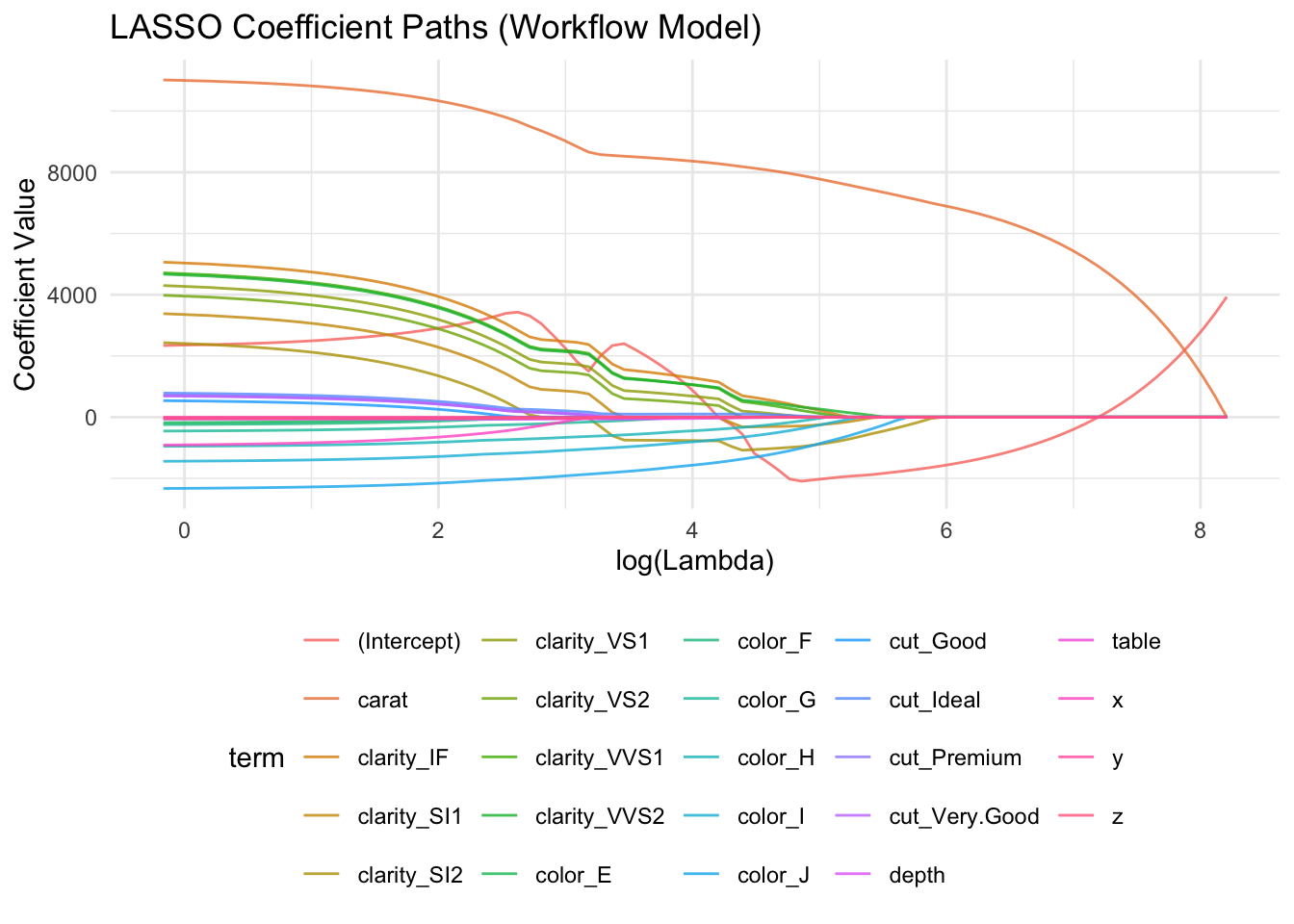
Here is a visualization of how the coefficients change with different parameters \(\lambda\).
Decision trees and the more general random forest methods provide other ways to predict. There are various packages to implement these methods in R, including rpart. One issue that arises in all these methods is overfitting. This means that the model performs very well in the training data, but not so well in the testing data. Cross-validation is a tool that addresses this issue. The basic idea of cross-validation is that the split of the data is not so simplistic into training/testing. Instead, the data is repeatedly divided into multiple subsets (or “folds”), so that each part of the data is used for both training and testing at different stages. For example, in 5-fold cross-validation, the data is split into five parts: the model is trained on four and tested on the fifth, and this process repeats five times. The average performance across all folds gives a more reliable estimate of how the model is likely to perform on new, unseen data.
21.2 Unsupervised Learning
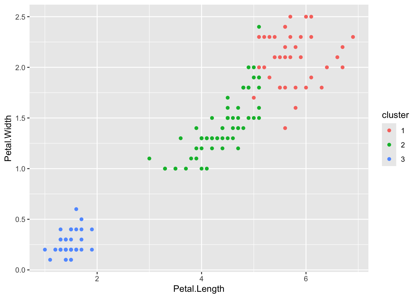
A common application of unsupervised learning is “clustering” or “pattern recognition.” The most foundational approach is the k-means algorithm, which attempts to group observations into \(k\) clusters based on similarity. The intuition behind k-means is simple: the algorithm assigns each observation to the nearest cluster center, then updates the cluster centers to be the average of the observations assigned to them. This process repeats until the assignments stop changing. The result is a division of the data into groups that are internally similar but distinct from one another. While it is fast and widely used, it does require the user to specify the number of clusters in advance. K-means and similar tools are useful for summarizing large datasets, detecting outliers, or identifying natural groupings when no outcome variable is available.
# Remove the species label for unsupervised learningiris_data <- iris[, 1:4]# Run k-means with 3 clusters (we know there are 3 species)set.seed(470500)iris_kmeans <-kmeans(iris_data, centers =3, nstart =20)# Add the cluster labels to the original datairis_clustered <- iris %>%mutate(cluster =as.factor(iris_kmeans$cluster))# Plot the clusters (e.g., using petal length vs. width)library(ggplot2)ggplot(iris_clustered, aes(x = Petal.Length, y = Petal.Width, color = cluster)) +geom_point()
21.3 Further Reading
There are so many great resources online to learn ML methods. Athey and Imbens (2019) provides a nice overview on the classes of methods. Text analysis is another class of machne learning that is useful. You can use the libraries tidytext or tm for that.