Before discussing difference-in-differences, it is important to understand the terminology for data that extends over time.
Cross-sectional data. In this type of data, there is one observation per unit. This is the type of data we have been considering in the class so far.
Panel data. In this type of data, there are multiple observations per unit corresponding to multiple time periods. This is the type of data we will consider for difference-in-differences. Another name for panel data is longitudinal data.
Like before, we use \(i\) to index the units of the dataset (individuals, households, firms, counties, countries, etc.). Unlike before, we also have to index time periods, \(t\). Time periods can be anything: years, seconds, decades, etc. It is convenient to consider there are \(N\) individuals, so that \(i = 1, 2, \ldots, N\), and \(T\) time periods, so that \(t = 1, 2, \ldots, T\).
The advantage of panel data is that it allows us to consider a “before and after” something changes. We can then see the effect of a policy intervention by comparing what happens after the intervention to what happens before the intervention.
We can load an example panel dataset from the AER package.
library(AER)
Loading required package: car
Loading required package: carData
Loading required package: lmtest
Loading required package: zoo
Attaching package: 'zoo'
The following objects are masked from 'package:base':

    as.Date, as.Date.numeric
Loading required package: sandwich
Loading required package: survival
library(dplyr)
Attaching package: 'dplyr'
The following object is masked from 'package:car':

    recode
The following objects are masked from 'package:stats':

    filter, lag
The following objects are masked from 'package:base':

    intersect, setdiff, setequal, union
library(ggplot2)library(magrittr)library(tidyr)
Attaching package: 'tidyr'
The following object is masked from 'package:magrittr':

    extract
data(Fatalities)# Explore the data (commented to be concise)# summary(Fatalities)
This dataset contains the number of deaths from traffic accidents in the continental U.S. annually from 1982 to 1988. Before we dive in, answer the following questions about the data.
What is the unit of analysis in the data?
What is the unit of time period in the data?
How many observations and variables are there?
Is the dataset in long or wide format?
A policymaker might be interested in the relationship between traffic fatalities and taxes on alcohol. We can use this dataset to see the relationship. To begin, let us look at a naive correlation between the fatality rate and the tax on beer.
# Calculate the fatality rate per 10,000 peopledf <- Fatalities %>%mutate(frate = fatal / pop *10000)summary(df$frate)
   Min. 1st Qu.  Median    Mean 3rd Qu.    Max.
 0.8212  1.6237  1.9560  2.0404  2.4179  4.2178
# Correlation in 1982lm(frate ~ beertax, data =filter(df, year ==1982)) %>%summary()
Call:
lm(formula = frate ~ beertax, data = filter(df, year == 1982))

Residuals:
    Min      1Q  Median      3Q     Max
-0.9356 -0.4480 -0.1068  0.2295  2.1716

Coefficients:
            Estimate Std. Error t value Pr(>|t|)
(Intercept)   2.0104     0.1391  14.455   <2e-16 ***
beertax       0.1485     0.1884   0.788    0.435
---
Signif. codes:  0 '***' 0.001 '**' 0.01 '*' 0.05 '.' 0.1 ' ' 1

Residual standard error: 0.6705 on 46 degrees of freedom
Multiple R-squared:  0.01332,   Adjusted R-squared:  -0.008126
F-statistic: 0.6212 on 1 and 46 DF,  p-value: 0.4347
# Correlation in 1988lm(frate ~ beertax, data =filter(df, year ==1988)) %>%summary()
Call:
lm(formula = frate ~ beertax, data = filter(df, year == 1988))

Residuals:
     Min       1Q   Median       3Q      Max
-0.72931 -0.36028 -0.07132  0.39938  1.35783

Coefficients:
            Estimate Std. Error t value Pr(>|t|)
(Intercept)   1.8591     0.1060  17.540   <2e-16 ***
beertax       0.4388     0.1645   2.668   0.0105 *
---
Signif. codes:  0 '***' 0.001 '**' 0.01 '*' 0.05 '.' 0.1 ' ' 1

Residual standard error: 0.4903 on 46 degrees of freedom
Multiple R-squared:  0.134, Adjusted R-squared:  0.1152
F-statistic: 7.118 on 1 and 46 DF,  p-value: 0.0105
Our results are counter-intuitive. It seems that increasing taxes actually increases fatality rate. While this may be the case, we cannot conclude anything causal due to omitted variable biases. We have some covariates in this dataset that my help us control for economic conditions, demographic factors, etc., but we may always be concerned about unobservable factors that determine traffic fatalities, some of which may be related to alcohol taxes. Fixed effects can help us!
19.2 Fixed Effects
We can consider all the observable and unobservable factors of unit that do not vary over time using unit fixed effects. These are just indicator variables for each of the states.
If \(Y_{it}\) is the fatality rate for state \(i\) in year \(t\) and \(X_{it}\) is the tax for beer, then we can think of the following regressions for 1982 and 1988 with fixed effects:
Notice that because the fixed effects do not vary over time, if we take the difference of the two equations then the fixed effects will cancel out. This will help us capture the correlation between changes in taxes and changes in traffic fatalities:
Call:
lm(formula = frate_diff ~ beertax_diff, data = df_wide)

Residuals:
     Min       1Q   Median       3Q      Max
-1.22715 -0.09619  0.09212  0.22290  0.67745

Coefficients:
             Estimate Std. Error t value Pr(>|t|)
(Intercept)  -0.07204    0.06064  -1.188   0.2410
beertax_diff -1.04097    0.41723  -2.495   0.0162 *
---
Signif. codes:  0 '***' 0.001 '**' 0.01 '*' 0.05 '.' 0.1 ' ' 1

Residual standard error: 0.394 on 46 degrees of freedom
Multiple R-squared:  0.1192,    Adjusted R-squared:    0.1
F-statistic: 6.225 on 1 and 46 DF,  p-value: 0.01625
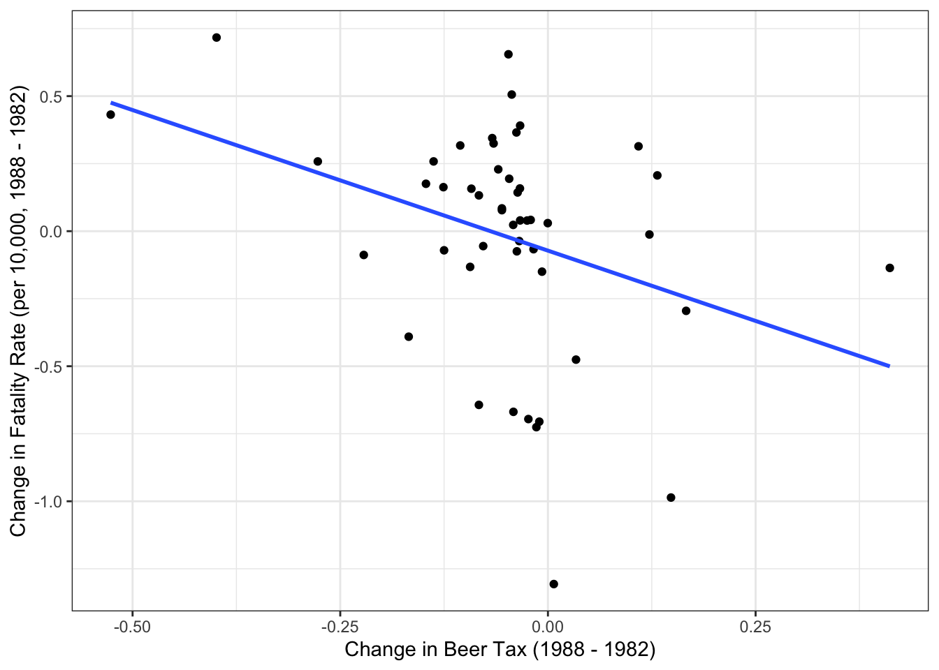
Now we see that when we increase the beer tax, that is correlated with a change in fatality rates. Increasing the tax on a case of beer by one dollar results in 1.04 deaths per 10,000 people on average. We can evaluate the magnitude of this by looking at the summary statistics of the outcome variable and considering the data. This effect seems pretty large. Even with taking the differences to remove the time-invariant, state-level factors, there could be other omitted variables that make the change in beer tax endogenous.
ggplot(data = df_wide) +geom_point(aes(x = beertax_diff, y = frate_diff)) +geom_smooth(aes(x = beertax_diff, y = frate_diff), method ="lm", se =FALSE) +labs(x ="Change in Beer Tax (1988 - 1982)",y ="Change in Fatality Rate (per 10,000, 1988 - 1982)") +theme_bw()
   frate_1982      frate_1988      frate_diff
 Min.   :1.101   Min.   :1.231   Min.   :-1.30657
 1st Qu.:1.618   1st Qu.:1.628   1st Qu.:-0.13319
 Median :2.046   Median :1.998   Median : 0.04075
 Mean   :2.089   Mean   :2.070   Mean   :-0.01951
 3rd Qu.:2.317   3rd Qu.:2.468   3rd Qu.: 0.23626
 Max.   :4.218   Max.   :3.236   Max.   : 0.71697
We can also consider regressions with the fixed effects without taking the differences between time periods. We call these panel regression models:
Notice that we have the state fixed effects (\(Z_i\)). You can imagine this regression for each \(t\) that we have in the data. The basic idea here is that each state has its own intercept (\(\beta_2 Z_i\)) in addition to the common intercept (\(\beta_0\)). The notation above is a bit of a shorthand for including indicators for each of the units except (arbitrarily) the first one:
If we remove the common intercept, then we can also include the intercept for the first unit.
Let us estimate the model with traffic fatalities and the beer tax. Notice that we want to use the long data. It is useful to compare with and without intercept. We see the coefficients of the fixed effects, but we are only interested in the estimated coefficient on the beer tax: \(-0.657\).
# With Interceptlm(frate ~ beertax + state, data = df) %>%summary()
While we can always use lm(), we can also use a package called plm to more conveniently estimate fixed effect regressions. The model is called “within” because we want there to be unit fixed effects. We get the same result but it does not show all the estimated coefficients for the fixed effects.
library(plm)
Attaching package: 'plm'
The following objects are masked from 'package:dplyr':

    between, lag, lead
plm(frate ~ beertax, data = df,index =c("state", "year"),model ="within") %>%summary()
Oneway (individual) effect Within Model

Call:
plm(formula = frate ~ beertax, data = df, model = "within", index = c("state",
    "year"))

Balanced Panel: n = 48, T = 7, N = 336

Residuals:
      Min.    1st Qu.     Median    3rd Qu.       Max.
-0.5869619 -0.0828376 -0.0012701  0.0795454  0.8977960

Coefficients:
        Estimate Std. Error t-value Pr(>|t|)
beertax -0.65587    0.18785 -3.4915 0.000556 ***
---
Signif. codes:  0 '***' 0.001 '**' 0.01 '*' 0.05 '.' 0.1 ' ' 1

Total Sum of Squares:    10.785
Residual Sum of Squares: 10.345
R-Squared:      0.040745
Adj. R-Squared: -0.11969
F-statistic: 12.1904 on 1 and 287 DF, p-value: 0.00055597
We still may not be satisfied with these estimates! What if there are factors that are changing over time, not just over states? We can include time fixed effects for this. I will use \(\delta_t\) to stand in for all the indicators:
We can run the below regressions because both state and year are factor variables. If they are not factor variables, then we need to convert them before running the regression.
# State fixed effectslm(frate ~ beertax + state -1, data = df) %>%summary()
For these regressions, we need to be careful with the standard errors. Normally, we assume homoskedasticity, and for longitudinal data, we do not want there to be correlation between the unobserved variables. However, \(U_{it}\) will naturally be correlated with \(U_{it+1}\) because they are both for the same unit. Similarly, \(U_{it}\) will be correlated with \(U_{jt}\) because they are both for the same time period.
We can cluster the standard errors to allow for heteroskedasticity and autocorrelated errors within the cluster, but not across clusters. To do, we can use plm so that we have a plm object rather than an lm object. Then, we can use coeftest() with the sandwich package to calculate the clustered standard errors.
library(sandwich)plm_out <-plm(frate ~ beertax,data = df,index =c("state", "year"),model ="within",effect ="twoways") # This does state and year fixed effectscoeftest(plm_out, vcov = vcovHC, type ="HC1")
t test of coefficients:

        Estimate Std. Error t value Pr(>|t|)
beertax -0.63998    0.35015 -1.8277  0.06865 .
---
Signif. codes:  0 '***' 0.001 '**' 0.01 '*' 0.05 '.' 0.1 ' ' 1
19.3 Difference-in-Differences
Now we are comfortable with panel data and fixed effects. In some cases, you may be comfortable assuming that the fixed effects account for all possible unobserved heterogeneity that could be correlated with the covariate of interest (e.g., beer taxes), and interpret the above estimates causally. This is hard to argue though, and there may be something better we can do: difference-in-differences.
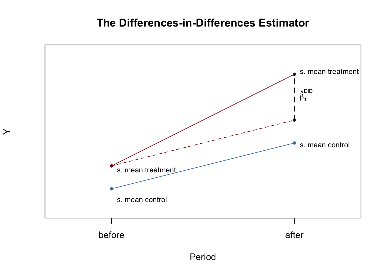
Suppose there is a large change in the taxes in Texas but a small change in the taxes in Oklahoma. If we compare Texas to Oklahoma in 1988, we will see the difference between the two states after the policy, but what if this is all due to differences between the states? If we compare Texas in 1982 to Texas in 1988, we may see a difference but what if this is all due to differences between the years? We can take the “difference-in-differences” to account for both possibilities and just see the change due to the policy change. Here are the means for each of the groups before (pre) and after (post) the policy:
df <-tibble(Y =c(y_pre, y_post),D =rep(TDummy, 2), Post =c(rep("1", N), rep("2", N)))lm(Y ~ D * Post, data = df) %>%summary()
Call:
lm(formula = Y ~ D * Post, data = df)

Residuals:
    Min      1Q  Median      3Q     Max
-2.8788 -0.6071 -0.0357  0.6399  3.8692

Coefficients:
            Estimate Std. Error t value Pr(>|t|)
(Intercept)   5.9209     0.1020  58.044   <2e-16 ***
D             1.2918     0.1443   8.955   <2e-16 ***
Post2         2.0414     0.1443  14.151   <2e-16 ***
D:Post2       3.9477     0.2040  19.350   <2e-16 ***
---
Signif. codes:  0 '***' 0.001 '**' 0.01 '*' 0.05 '.' 0.1 ' ' 1

Residual standard error: 1.02 on 396 degrees of freedom
Multiple R-squared:  0.8816,    Adjusted R-squared:  0.8807
F-statistic: 982.9 on 3 and 396 DF,  p-value: < 2.2e-16
The key assumption is commonly called “parallel trends.” This boils down to: in the absence of treatment, the trends of the treatment and the control group would be the same. We can see this most easily in the graph. This means that there cannot be unobserved factors that vary by time and by unit that are correlated with treatment.
19.4 Further Reading
These notes are based on chapters 10 and 13 of Hanck et al. (2018). See that source for more information.
19.4.1 References
Hanck, Cristoph, Martin Arnold, Alexander Gerber, and Martin Schmelzer. 2018. Introduction to Econometrics with R. https://bookdown.org/machar1991/ITER/.